Photometric graphs

The React graphs render SVG without creating a GPU context. They consume the same Type C IESProfile as the viewer. Their calculation and geometry APIs live in @ies-tools/core, which has no React, Three.js or DOM dependency and works in Node. @ies-tools/viewer/graphs re-exports them for compatibility, alongside the viewer's presentation helpers (graphFrame, heatColor).

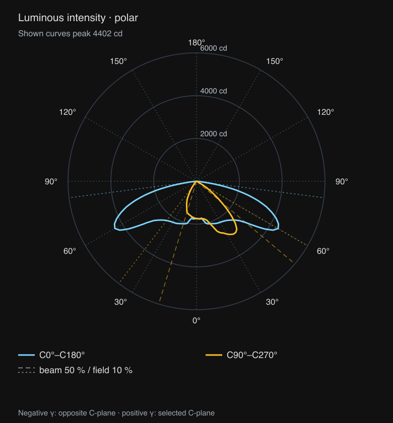
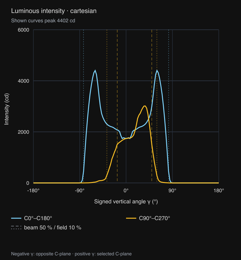
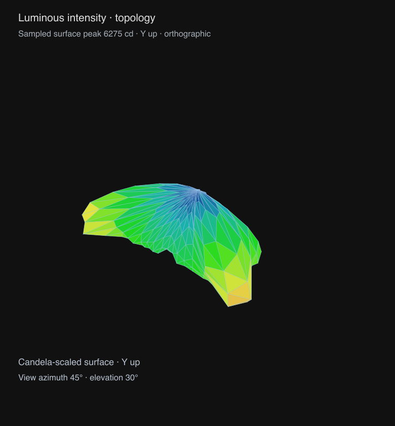
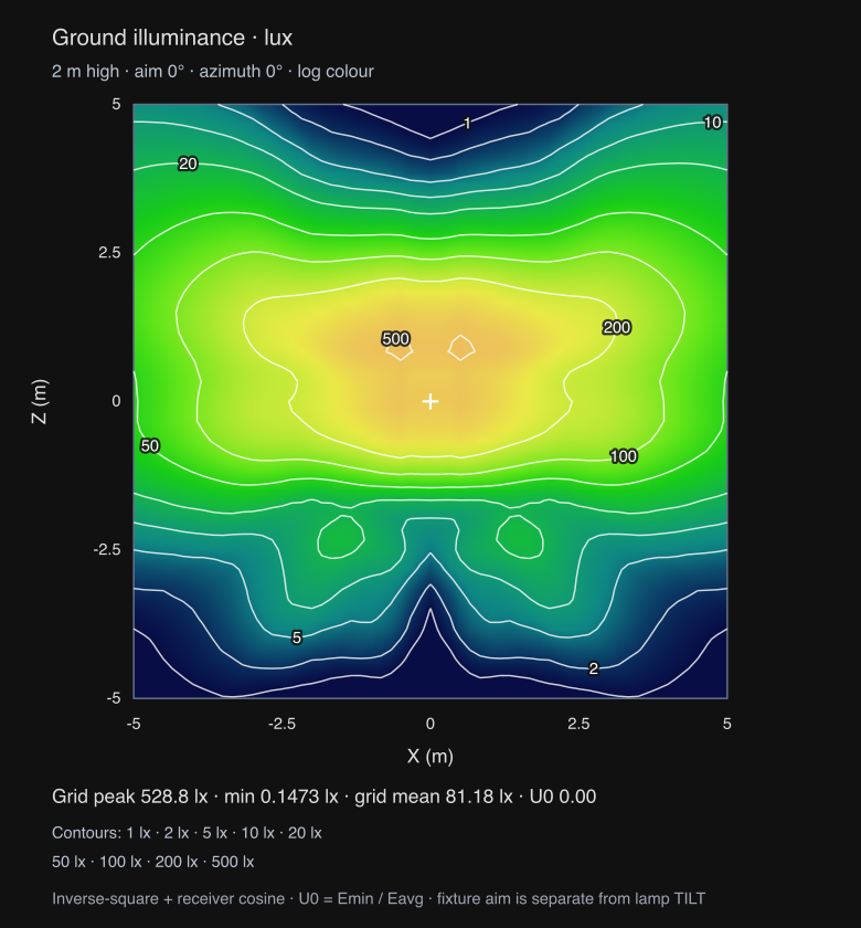
The same graphs, exported from an asymmetric BEGA luminaire with ies chart:

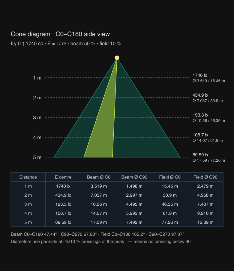
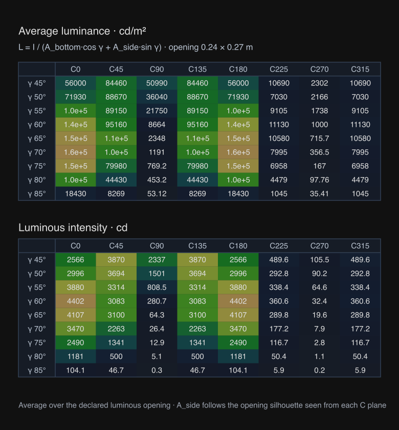
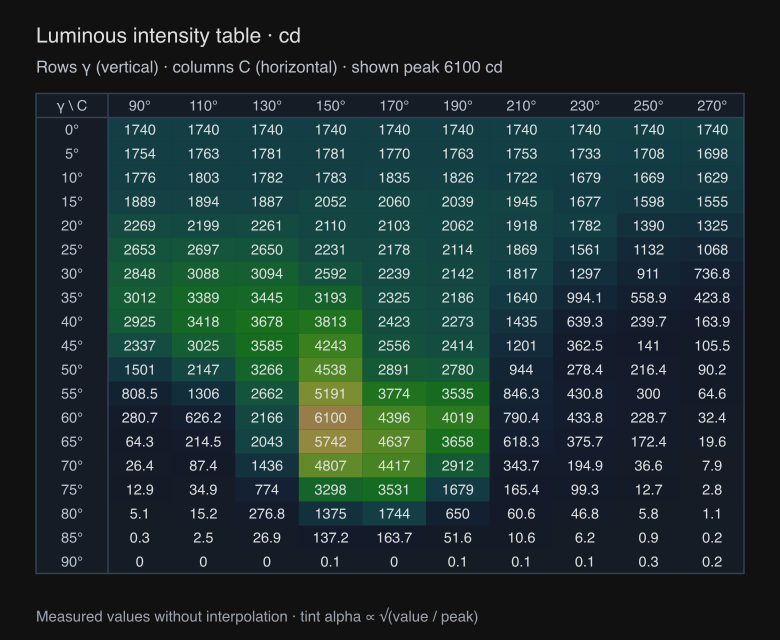
Complete intensity cuts

import { IntensityGraph } from '@ies-tools/viewer/react';

// Full C0–C180 and C90–C270 principal-plane curves, on one shared scale.
<IntensityGraph profile={profile} principalPlanes />;

// Three complete cuts overlaid on labeled Cartesian axes.
<IntensityGraph profile={profile} projection="cartesian" planes={[0, 45, 90]} />;

// Sweep horizontal C at three fixed vertical angles.
<IntensityGraph profile={profile} axis="horizontal" planes={[30, 60, 90]} />;

axis, angle and upAxis retain their existing meanings. For a vertical sweep, a complete cut samples C=angle on the positive side of gamma and C=angle + 180° on the negative side. Both sides use actual measurements; the graph does not mirror one side to manufacture a symmetric distribution. The default shows one complete cut at C0–C180. principalPlanes selects C0–C180 and C90–C270 when planes is omitted. Explicit planes always takes precedence.

For horizontal sweeps, angle or each entry in planes is the fixed vertical angle, and C sweeps 0–360°. Plane lists contain one to eight angles. Angles are degrees; intensity is absolute candela, not peak-normalized attenuation.

The requested uniform samples are supplemented by measured angle knots, including symmetry-expanded horizontal knots. This preserves narrow peaks on irregular input grids. samples defaults to 361, ranges from 3 to 1441, and must be odd for vertical cuts so the curve includes nadir. The caption reports the peak of the shown curves, which can differ from the maximum over every measured C-plane. Cartesian views include labeled angles, candela ticks and curve legends; polar views include radial candela scales and dotted spokes labelled every 30°.

Vertical cuts also carry curve.beam, the getBeamAngles estimate for that opposed-plane cut. Both charts draw its 50 % (beam, dashed) and 10 % (field, dotted) crossings on each side of the peak in a muted copy of the curve colour, as radial lines on the polar chart and vertical lines on the Cartesian chart. A cut whose status is not ok gets no markers.

// Three decades on a log scale: radius = log10(I / Imin) / 3 × R, with Imin = Imax / 1000.
<IntensityGraph profile={profile} principalPlanes logScale />

logScale applies to polar and Cartesian views. Intensities at or below Imin sit at the centre (or the Cartesian baseline), and the rings or ticks fall on 1-2-5 candela values in each decade. logRadius and logTicks from @ies-tools/core expose the same mapping. The light viewer's chart tabs have a Log scale checkbox, and ies chart --log-scale exports the same view.

Intensity topology

<IntensityGraph
  profile={profile}
  projection="topology"
  upAxis="z"
  topologyProjection="perspective"
  viewAzimuth={35}
  viewElevation={25}
  surface="both"
  horizontalSegments={48}
  verticalSegments={48}
/>

The topology is a full candela-scaled surface, projected to SVG. surface is filled, wireframe, or both (default); colors encode intensity. Filled triangles are painted from far to near. topologyProjection is orthographic (default) or perspective; the default 45° azimuth and 30° elevation provide an isometric-style view. upAxis rotates the chosen source axis upward while preserving handedness. View azimuth ranges from −360° to 360° and elevation from −90° to 90°.

horizontalSegments defaults to 36 and ranges from 4 to 144; verticalSegments defaults to 36 and ranges from 2 to 144. Unlike the curve plots, topology uses a regular resampled angular grid: increase its resolution for very narrow features. Its caption reports the sampled surface peak, rather than claiming the global measured peak. This is a surface diagram with depth-sorted triangles, rather than a 3D renderer with a depth buffer.

Ground illuminance / isolux

import { IsoluxGraph } from '@ies-tools/viewer/react';

<IsoluxGraph
  profile={profile}
  mountingHeight={3}
  extent={[12, 8]}
  resolution={61}
  aimAngle={30}
  azimuth={90}
  contourLevels={[5, 10, 20, 50]}
/>;

The calculation places the fixture at (0, mountingHeight, 0) above a ground plane at Y=0. Aiming rotates the receiver direction into the luminaire's measured coordinate frame before sampling intensity. Ground illuminance is:

lux = I(local direction in candela) × receiver cosine / distance²

aimAngle is the angle away from nadir toward azimuth. Zero points down. azimuth runs from +X toward +Z and also turns the C0 plane. Ground coordinates X/Z and mounting height use metres. The map includes a marker directly below the luminaire, physical axes, labelled lux contours and sampled-grid statistics: peak, minimum, mean and uniformity U0 = Emin / Eavg. The reported grid mean is an arithmetic mean of grid points, not an integrated area average. The heatmap is a smooth bilinear fill: one PNG pixel per grid point, upscaled by the SVG renderer, so it needs no canvas and exports to SVG and PNG alike. Contour labels are placed greedily along each line, as far as possible from labels already placed; a label that would overlap another is omitted, and the legend still lists every drawn level.

Prop	Meaning and bounds
mountingHeight	Metres above ground; default 2; 0.01–10,000
extent	Full ground width/depth, centered below the fixture; number for a square or [width, depth]; default 10 m; each dimension 0.01–100,000 m
resolution	Points per axis, rather than cells; number or [columns, rows]; default 51; integer 2–201
aimAngle	Fixture aiming away from nadir, 0–180°; default 0
azimuth	Fixture/C0 orientation, −360–360°; default 0
lampTilt	Separate lamp-dependent IES TILT correction angle, −180–180°; default 0
contourLevels	Strictly increasing absolute lux levels; at most 32; omitted uses the 1-2-5 series; [] hides contours (contours is a deprecated alias)
minContour	Lowest automatic 1-2-5 level in lux; default 1. Levels run up to the largest value below the grid peak, at most 10, dropping the lowest
colorScale	log (default) maps colour logarithmically from the lowest level to the peak, so 1–50 lx spill stays visible; linear maps lux to peak
heatmap	Display the colored receiver grid; default true
className, style	SVG styling

Fixture aiming is a geometric rotation. It does not automatically change the lamp-dependent IES TILT correction. If the fixture's lamp correction requires a particular angle, pass it independently as lampTilt; intensity graphs accept the same correction prop. The workbench's isolux controls affect the footprint calculation; the 3D scene retains its downward-facing fixture.

This is direct illumination from measured angular intensity. It does not simulate indirect light, occlusion, luminaire aperture near-field effects, or room reflections. Type A/B data are rejected until a validated coordinate transform is available. Invalid dimensions, angles, sample counts and contour grids throw descriptive errors instead of producing invalid SVG.

Cone diagram, glare luminance and intensity tables

import { ConeDiagramGraph, IntensityTableGraph, LuminanceTableGraph } from '@ies-tools/viewer/react';

<ConeDiagramGraph profile={profile} maxDistance={6} />;
<LuminanceTableGraph profile={profile} />;
<IntensityTableGraph profile={profile} unit="cd/klm" maxColumns={12} />;

These three charts are Type C only; other photometric types render an "available for Type C photometry only" message instead of values.

Cone diagram. For distances 1…maxDistance metres (default 5, integer 1–50; or explicit distances), the centre illuminance is E = I(γ = 0) / d² on a plane facing the luminaire. Beam (50 %) and field (10 %) diameters use the per-side crossings reported by getBeamAngles (beamLeftDegrees, beamRightDegrees, fieldLeftDegrees, fieldRightDegrees; signed vertical angles, negative in the opposite C-plane) in the C0–C180 and C90–C270 planes: Ø = d · (tan right − tan left), which equals d · (tan|left| + tan|right|) for crossings on both sides of nadir. A diameter is shown as — when a crossing is missing or at/after 90°. The SVG shows the C0–C180 side view with the beam and field cones plus a table of distance, E centre and the four diameters.

Glare-angle luminance. Average luminance L(C, γ) = I(C, γ) / A_proj in cd/m² over the luminous opening declared in the file, for γ = 45°, 50°, …, 85° and C = 0°, 45°, …, 315° (override with gammas and cPlanes). A_proj = A_bottom · cos γ + A_side(C) · sin γ. Dimensions are converted from feet when needed. IES length runs along C0–C180 and width along C90–C270, so a rectangular opening's side silhouette from plane C is height × (width·|cos C| + length·|sin C|). A negative width declares a circular opening of diameter |width|, with bottom area π·d²/4 and side area height × d. A second table shows the sampled intensity at the same angles. A zero luminous area shows a message instead of luminance values. Intensity is sampled with the same interpolation as the other charts.

Intensity table. The measured candela grid with γ rows and C columns, in cd or cd/klm (normalized by the declared lamp flux; absolute photometry stays in cd). Each cell has a subtle heat-map tint with alpha ∝ √(value / peak). Cells keep a readable minimum width, so large grids widen the SVG; the viewer tab scrolls it. For fixed-size images, maxColumns and maxRows keep evenly spaced angles, always including the first and last.

Calculation and geometry APIs

The chart data builders are part of @ies-tools/core. Use them to draw the same charts with another renderer or to export the values:

import {
  buildIntensityCurves,
  buildIntensityTopology,
  buildIsoluxGrid,
  groundIlluminance,
  extractContours,
  isoluxContourLevels,
  niceTicks,
  buildConeDiagram,
  buildLuminanceTable,
  buildIntensityTable,
} from '@ies-tools/core';

const cuts = buildIntensityCurves(profile, { principalPlanes: true });
// cuts.curves[].points: { angle: signed degrees, intensity: candela }
// cuts.angleTicks and cuts.intensityTicks are ready for a custom chart.

const mesh = buildIntensityTopology(profile, { upAxis: 'z', projection: 'orthographic' });
// vertices[].position: actual candela-scaled XYZ; projected: normalized XY, positive Y up.
// faces: triangle index triples, sorted far to near. Caller can use a different renderer.

const lux = groundIlluminance(profile, 1, 2, { mountingHeight: 3, aimAngle: 30 });
const grid = buildIsoluxGrid(profile, { mountingHeight: 3, extent: [12, 8], resolution: [61, 41] });
// grid.xs, grid.zs, grid.values[zIndex][xIndex], maximum, minimum, average and uniformity (U0).
const levels = isoluxContourLevels(grid.maximum, { minContour: 1 }); // [1, 2, 5, 10, 20, 50, …]
const contours = extractContours(grid, levels);
// contours[].segments: [[x1, z1], [x2, z2]] in physical ground coordinates.
const ticks = niceTicks(grid.maximum);

const cone = buildConeDiagram(profile, { maxDistance: 5 });
// cone.rows[]: { distance, illuminance, beamDiameters: [c0, c90], fieldDiameters: [c0, c90] }
const glare = buildLuminanceTable(profile);
// glare.luminance[gammaIndex][cIndex] in cd/m² (null for zero area); glare.intensity in cd.
const table = buildIntensityTable(profile, { unit: 'cd/klm' });
// table.values[gammaIndex][cIndex], with table.gammas, table.cPlanes and table.unit.

extractContours uses marching squares with linearly interpolated edge crossings and a center-value saddle decision. Flat fields and exact-corner degeneracies produce no zero-length segments. Segments are unstitched so consumers can render or join them as appropriate. The grid and contour approximation improves with resolution; it is not an analytic boundary solver.